Pearson Correlation
A statistical technique to investigate the strength and direction of the relationship between two quantitative variables

Complete the form below to unlock access to ALL audio articles.
Pearson’s correlation is a commonly used statistical technique for investigating the strength and direction of the relationship between two quantitative variables, such as the relationship between age and height. In this article, we will explore the theory, assumptions and interpretation of Pearson’s correlation, including a worked example of how to calculate Pearson’s correlation coefficient, often referred to as Pearson’s r.
What is Pearson correlation test, Pearson product moment correlation or Pearson r?
Scatter plots
Pearson correlation coefficient formula
What are the assumptions of Pearson's correlation test?
Pearson vs Spearman correlation and when to use Pearson's r
Pearson’s correlation coefficient interpretation
Pearsons R test example
What is Pearson correlation test, Pearson product moment correlation or Pearson r?
Pearson’s correlation helps us understand the relationship between two quantitative variables when the relationship between them is assumed to take a linear pattern. The relationship between two quantitative variables (also known as continuous variables), can be visualized using a scatter plot, and a straight line can be drawn through them. The closeness with which the points lie along this line is measured by Pearson’s correlation coefficient, also often denoted as Pearson’s r, and sometimes referred to as Pearson’s product moment correlation coefficient or simply the correlation coefficient. Pearson’s r can be thought of not just as a descriptive statistic but also an inferential statistic because, as with other statistical tests, a hypothesis test can be performed to make inferences and draw conclusions from the data.
Scatter plots
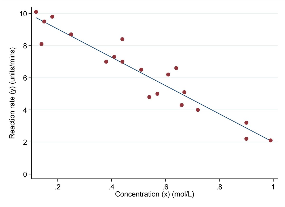
A common first step when investigating the relationship between two quantitative variables is to plot the data in a scatter diagram, where the outcome (response or dependent) variable is on the vertical y-axis and the exposure (explanatory or independent) variable is on the horizontal x-axis, with markers representing the values of each variable an individual takes in the dataset. An example of a scatter plot can be found in Figure 3.
Pearson correlation coefficient formula
The formula for Pearson’s correlation coefficient, r, relates to how closely a line of best fit, or how well a linear regression, predicts the relationship between the two variables. It is presented as follows:

where xi and yi represent the values of the exposure variable and outcome variable for each individual respectively, and x̄ and ȳ represent the mean of the values of the exposure and outcome variables in the dataset.
This formula works by numerically expressing the variation in the outcome variable “explained” by the exposure variable. In essence, we are calculating the sum of products (multiplying corresponding values from pairs and then adding together the resulting values) about the mean of x and y divided by the square root of the sum of squares about the mean of x multiplied by the sum of squares about the mean of y. The variation is expressed using the sum of the squared distances (e.g. (xi – x̄)2) of the values from the mean of y and x. This captures the variation in the values around the line of best fit and also ensures the correlation coefficient lies between − 1 and + 1.
What are the assumptions of Pearson's correlation test?
There are some key assumptions that should be met before Pearson’s correlation can be used to give valid results:
- The data should be on a continuous scale. Examples of continuous variables include age in years, height in centimeters and temperature in degrees Celsius. Sometimes continuous variables are referred to as quantitative variables, although, it’s important to remember that, while all continuous variables are quantitative, not all quantitative variables are continuous.
- The variables should take a Normal distribution. This assumption means the Pearson’s correlation test is a parametric test. If the data in the variables of interest take some other distribution, then a non-parametric test for correlation such as Spearman’s rank correlation should be used. This assumption can be checked using a histogram.
- There should be no outliers in the dataset. Outliers are values that are notably different from the pattern of the rest of the data and may influence the line of best fit and warp the correlation coefficient.
- The relationship between the two variables is assumed to be linear. This assumption is related to the “no outliers” assumption, in that the relationship should be able to be described by a straight line relatively well. These assumptions can be checked using scatter plots (Figure 1).

Figure 1: Scatter plots showing examples of linear and non-linear relationships. Credit: Technology Networks.
Pearson vs Spearman correlation and when to use Pearson's r
Pearson’s correlation and Spearman’s rank correlation share the same purpose of quantifying the strength and direction (negative or positive) of an association between two variables. The correlation coefficients can be used to conduct a hypothesis test for the strength of evidence for the correlation between two variables of interest.
Unlike Spearman’s correlation, Pearson’s correlation assumes normality and a linear relationship between the variables. Spearman’s correlation test is non-parametric and assumes neither a specific distribution nor a linear relationship, so it is suitable when these assumptions are not met. Pearson’s correlation is based on standard deviation and covariance of datapoints around a best fit line, whereas Spearman’s rank correlation is based on ranking data points and is suitable only for measuring monotonic association (as one variable increases (or decreases) the other variable also increases (or decreases)).
Pearson’s correlation coefficient interpretation
The properties and interpretation of Pearson’s r can be summarized as follows:
- r always lies between − 1 and + 1.
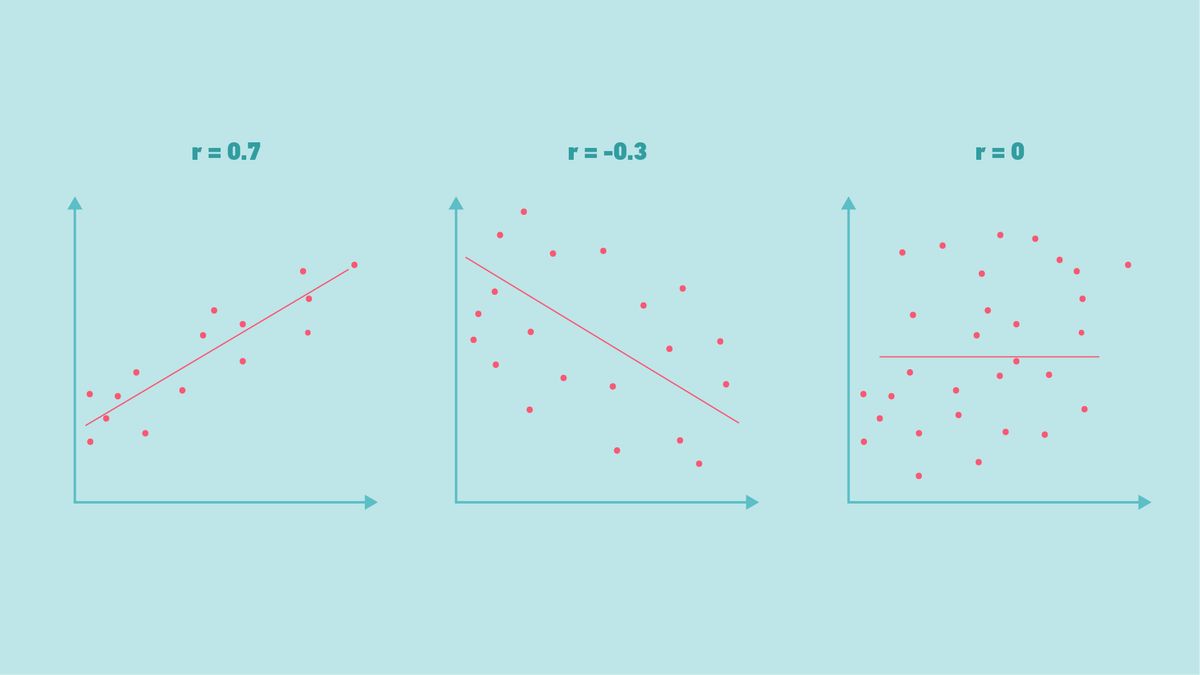
- Positive correlation (positive values of r) is when one variable increases and the other tends to increase. Negative correlation (negative values of r) is when one variable decreases and the other tends to increase. See Figure 2 for some examples.
- Values closer to − 1 and + 1 indicate stronger relationships and r will be equal to 0 when variables are not linearly associated, with − 1 and + 1 representing when the points are perfectly on the line of best fit. It should be noted that the variables may still be associated if r = 0, but in a more complex, non-linear way.
- The more random the scatter of points around the line, the less correlated the data and the closer to 0 the value of r will be.
It is important to note that correlation coefficients assess only two variables at a time and should not be interpreted as causal relationships, where additional variables and multivariable methods are needed.

Figure 2: Scatter plots showing various relationships between two variables and their corresponding Pearson correlation coefficients, r. Credit: Technology Networks.
Pearsons R test example
Suppose a team of chemists is interested in the relationship between a reactant’s concentration (in mol/L) and reaction rate (in units/min). Both variables take a Normal distribution and the relationship is assumed to be linear, so a Pearson’s correlation test is appropriate (Figure 3). In this section we will calculate Pearson’s r using the formula by hand, but in reality, these calculations can be done for us using statistical software.

Figure 3: Scatter plot showing reactant concentration (x) and reaction rate (y) in our worked example, with a best fit line included. Credit: Elliot McClenaghan.
For the by-hand calculation, so that we can follow the steps clearly in our dataset, we can rearrange the formula as follows, where n is the number of observations or data points:


We need to calculate the sum of the x and y values, calculate x2 and y2, and their sums as well. Finally, the sum of the cross product (values of x multiplied by y). The raw values for each observation and the calculated values are shown in Table 1.
Table 1: Reactant concentration (x) and reaction rate (y) values required to calculate Pearson’s correlation coefficient, along with x2, y2 and the cross-product values. The sum (Σ) of each column is included in the bottom row.
| Observation | Concentration, x (mol/L) | Reaction rate, y (units/min) | x2 | y2 | x*y |
| 1 | 0.12 | 10.1 | 0.0144 | 102.01 | 1.212 |
| 2 | 0.25 | 8.7 | 0.0625 | 75.69 | 2.175 |
| 3 | 0.38 | 7 | 0.1444 | 49 | 2.66 |
| 4 | 0.51 | 6.5 | 0.2601 | 42.25 | 3.315 |
| 5 | 0.64 | 6.6 | 0.4096 | 43.56 | 4.224 |
| 6 | 0.66 | 4.3 | 0.4356 | 18.49 | 2.838 |
| 7 | 0.9 | 3.2 | 0.81 | 10.24 | 2.88 |
| 8 | 0.99 | 2.1 | 0.9801 | 4.41 | 2.079 |
| 9 | 0.15 | 9.5 | 0.0225 | 90.25 | 1.425 |
| 10 | 0.44 | 8.4 | 0.1936 | 70.56 | 3.696 |
| 11 | 0.41 | 7.3 | 0.1681 | 53.29 | 2.993 |
| 12 | 0.54 | 4.8 | 0.2916 | 23.04 | 2.592 |
| 13 | 0.67 | 5.1 | 0.4489 | 26.01 | 3.417 |
| 14 | 0.72 | 4 | 0.5184 | 16 | 2.88 |
| 15 | 0.9 | 2.2 | 0.81 | 4.84 | 1.98 |
| 16 | 0.18 | 9.8 | 0.0324 | 96.04 | 1.764 |
| 17 | 0.14 | 8.1 | 0.0196 | 65.61 | 1.134 |
| 18 | 0.44 | 7 | 0.1936 | 49 | 3.08 |
| 19 | 0.57 | 5 | 0.3249 | 25 | 2.85 |
| 20 | 0.61 | 6.2 | 0.3721 | 38.44 | 3.782 |
| Σ | Σx = 10.22 | Σy = 125.9 | Σx2 = 6.5124 | Σy2 = 903.73 | Σxy = 52.976 |
Step two is to calculate the Pearson’s correlation coefficient, r, using the formula, the calculated parameters and our sample size (n = 20).


In our example, we find Pearson’s correlation coefficient to be r = − 0.94. We can interpret this as evidence of strong negative correlation given that r is a negative value and close to − 1.
Step three is to conduct a hypothesis test for the relationship between the two variables using Pearson’s r.
As with other correlation tests and statistical tests, we can conduct a hypothesis test for the strength of evidence of the correlation and to assess to what extent our finding could be attributed to chance. Our hypotheses for the test are as follows:
- Null hypothesis (H0) is that the two variables are independent, that there is no linear relationship.
- Alternative hypothesis (H1) is that there is a linear relationship between the two variables, and that there is correlation.
We calculate our test statistic (t) by plugging in our r value and n into the following formula:


Next, we can use the degrees of freedom (df) (df is the number of independent bits of information in a statistical model or test; for Pearson correlation, the formula for this is df = n − 2), the significance level of interest (normally α = 0.05) and whether we are interested in a one-sided or two-sided test, to find a corresponding critical value of t using a t-distribution table. The t-distribution is a probability distribution that gives the probabilities of the occurrence of different outcomes for an experiment and is commonly used in statistical hypothesis testing.
The two-sided p-value is usually of more interest as it gives both directions of the effect and better represents the hypotheses of our test. In our example, we find a two-sided p-value of p < 0.001. This p-value indicates strong evidence against the null hypothesis. Therefore, we conclude that there is evidence of a negative correlation between the two variables, as reactant concentration increases, reaction rate decreases.
Further reading
- Bland M. An Introduction to Medical Statistics (4th ed.). Oxford. Oxford University Press; 2015. ISBN:9780199589920
- Laerd Statistics. Pearson product-moment correlation. https://statistics.laerd.com/statistical-guides/pearson-correlation-coefficient-statistical-guide.php. Accessed April 3, 2024.


